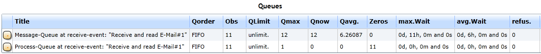
Figure 1 depicts the statistics table on the queues:
- Note that only the message receiving activity possesses queues.
- There are two queues.
- This is based on the following fact:
- Whenever a message or a process instance reaches an activity (that has an incoming message flow) there are two possibilities:
- Either the message is the first entity to arrive or the process instance.
- If the process instance arrives first, it will have to wait for a message to work off the activity.
- Otherwise if the message arrives first, it will have to wait for a process instance to pick it up.
- The latter construct is depicted in the table above.
- In our example model, the messages always arrive first.
- Therefore the message queue is the only one with significant statistical information for this model.
- As you can see, most of the process queue's values are zero, though we have got eleven Observations (of removing a process instance from the queue).
- But, let us check out the Zero column.
- Its value is also eleven.
- This means each of the eleven process instances (that have been put into the queue) have been removed instantly, because they did not have to wait for a message.
|
Figure 1: Queue statistics
|
But...
- On the other hand the message queue shows us the bottle-neck of this model.
- Here we have also got eleven observations, which is correct, because every time a process instance is being reactivated, it consumes one message (which will be removed from the message queue).
- Check out the other values:
- Currently there are twelve messages (Qnow) waiting to get picked up.
- This value matches the maximum number of elements (observed throughout the simulation).
- This indicates, that if we increase the simulation runtime, the maximum waiting time and with that the average waiting time will also increase.
- We can explain this correlation by having a look at the general simulation properties.
- The "Controlling"-process starts every time unit (Inter-arrival time = constantly 1),
- and the "Marketing"-process starts every second time unit (Inter-arrival time = constantly 2).
- So, we are sending twice as many messages as there are "Controlling"-process instances, which can receive the messages.
Note
- Of course there are models, where this principle of "always arriving first" is not valid and "gets mixed up" due to the stochastic influences on the model.
- E. g. change the inter-arrival time of our example model's both start events to
- a Normal Distribution with a mean value of 2 and a standard deviation value of 0.5.
- Check the report and you will notice, that both queues possess significant waiting times now.
See the table below for a description of the statistical elements of queues.
Queues
|
Title
|
Name of the queue.
|
Qorder
|
The Queuing order: FIFO (First in first out) is the default value and cannot be changed.
|
Obs
|
Observed removals of entities.
|
QLimit
|
The queue's limit (maximum number of entities this queue can contain). The default value is unlimited and cannot be changed.
|
Qmax
|
The maximum number of entities, this queue contained throughout the simulation.
|
Qnow
|
The current number of elements contained in this queue at the simulation stop.
|
Qavg
|
The average number of elements contained in this queue throughout the simulation.
|
Zeros
|
An element that is instantly removed from the queue without any time consumption is called a zero. (Zero for: spent 0 time units in the queue.)
|
max. Wait
|
This value represents the maximum waiting time of an element before getting removed from the queue.
|
avg. Wait
|
This value represents the average waiting time of an element before getting removed from the queue.
|
refus.
|
The number of elements that have been refused to be inserted into the queue.
|
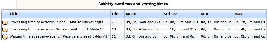
Activity run-times and waiting times of this model
The picture from below shows the model's activity run-times and waiting times.
|
Figure 2: Activity run-times and waiting times
|
- Contrary to our previous example models, we now have got a waiting time in the bottom row of the table.
- Its values (except the Obs) are 0.
- There is no time consumption, because our processes do not wait at this explicit activity.
- There is always a message available whenever a process instance arrives at the message receiving activity (see Zero column in the Queue statistics table).
- If we switch the inter-arrival time values of the two start events (like described above), there will be a non-zero waiting time.
- Since this model does not possess any further model dynamics, the activity's waiting time value should be equivalent to the process queue's waiting time values. Just try it out.