List of Stochastic Distributions

This section explains the stochastic distributions you can use in IYOPRO.

Constant Distribution

The constant value distribution has only one single possible value. There is therefore no “randomness”. In some cases this distribution can be very useful; e.g. for debugging and for comparisons of different distributions’ effects on simulation results.

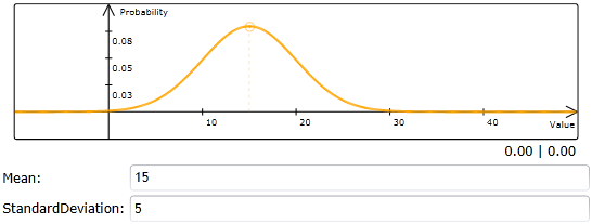
Normal Distribution
The normal distribution is the continuous counterpart of the Binomial or Poisson distribution. The sum of “sufficiently” many Bernoulli or Poisson distributed random processes (e.g. the number of customer arrivals during a given time span) approximates a normal distribution. The sum of measurement errors or the number of order completions of a machine with stochastic processing times provides good examples for this type of distribution.

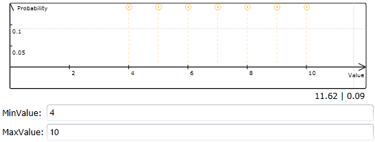
Discrete Uniform Distribution

The discrete uniform (or Laplace) distribution assigns the same probability to each of N events. It is often used where no better estimates can be given.

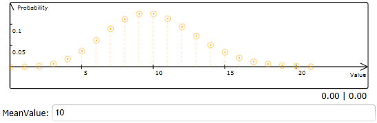
Poisson Distribution

A Poisson distribution approximates expected results of a binomial distribution well if probability is small and sample size is large. As long as the chosen interval is quite short, Poisson distributions can be successfully used to describe e.g. the number of arrivals of customer's telephone calls in a model.

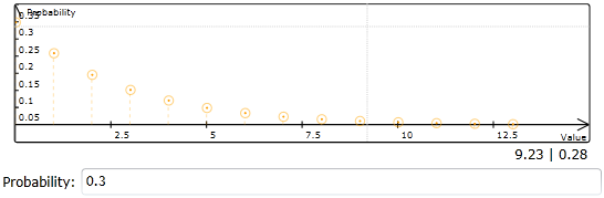
Geometric Distribution

The geometric distribution describes the probability that exactly k Bernoulli experiments will fail before the first success. For example, consider a production system in which a certain step can be described as Bernoulli experiment: The production step may fail, thus the success probability is p < 1. Assume that for each item produced this step is repeated until success. The number of repetitions necessary will be geometrically distributed.

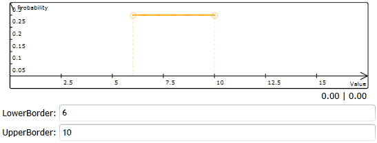
Continuous Uniform Distribution

Random numbers which follow a rectangular distribution (or continuous uniform distribution) are distributed over an interval, whose subintervals all have the same probability of occurrence. While this type of distribution is rare in reality, it is useful where no better knowledge is available and cannot be obtained with acceptable effort.

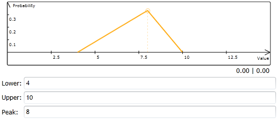
Triangular Distribution
In contrast to a rectangular distribution, in a triangular distribution values closer to the mode occur more probably than values near a or b. Triangularly distributed random numbers are also used where a part from other indications only knowledge about most frequent values (in addition to lower and upper bounds) is available. Capacity estimates for natural resources like coal mines or oil wells are an example.

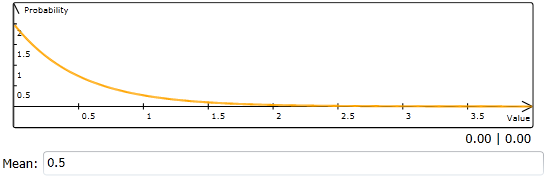
Exponential Distribution
The exponential distribution is the continuous counterpart of the geometric distribution. Inter-arrival times of customers or orders in systems without fixed time intervals typically follow exponential distributions.

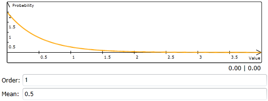
Erlang Distribution
The Erlang distribution is created by a aggregation of independent exponential distributions. In practice this is done by adding n exponentially distributed random numbers for each sample. Erlang distributions describe waiting times in a queuing system. Characterizing the life time of products or the length of time between system failures are other common examples for their application.

Empirical Distribution

The Empirical distribution assigns probabilities of appearance to empirically observed values. This distribution should be only used, if no other probability distribution fits with the given empirical data.